MLlib is the Spark is the primary library for addressing machine learning problem within the Spark ecosystem.

MLlib provides the following features:

• A collection of ML Algorithms for solving a variety of ML problem, such as classification, regression, clustering and collaborative filtering
• A collection of techniques for featurization, i.e., extracting and transforming the features of your dataset
• The ability to design e construct Pipeline of execution
• Persistence: models can be saved on file so that you will not be required to train a model every time you need to use it
• Utility tools, mostly for linear algebra e statistics

Spark MLlib is available in the version 3.0. It now uses dataset instead of regular RDDs.

In the following we will discuss some of the main tools provided by MLlib.

The code for this lesson is available here.

Basic Statistics

Correlation

Correlation measures the strength of a linear relationship between two variables. More specifically, given two variables X e Y, they are considered:

• positively correlated – if when X increases Y increases and vice versa
• negatively correlated – if when X increases Y increases and vice versa
• no correlated – when their trends are not dependent from one another

The quantity compute by MLLlib is the Pearson’s coefficient, which is defined in [-1,1]. A coefficient equal to 1 (-1) defines a strong positive (negative) correlation.

The following snippet compute the correlation matrix between each pair of variables.

import org.apache.spark.ml.linalg.{Matrix, Vectors}
import org.apache.spark.ml.stat.Correlation
import org.apache.spark.sql.Row

val data = Seq(
  Vectors.sparse(4, Seq((0, 1.0), (3, -2.0))),
  Vectors.dense(4.0, 5.0, 0.0, 3.0),
  Vectors.dense(6.0, 7.0, 0.0, 8.0),
  Vectors.sparse(4, Seq((0, 9.0), (3, 1.0)))
)

val df = data.map(Tuple1.apply).toDF("features")
val Row(coeff1: Matrix) = Correlation.corr(df, "features").head
println(s"Pearson correlation matrix:\n $coeff1")

val Row(coeff2: Matrix) = Correlation.corr(df, "features", "spearman").head
println(s"Spearman correlation matrix:\n $coeff2")

Summarizer

It provides a summary of the main statistics for each column of a given DataFrame. The metrics computed by this object are the column-wise:

• max

• min

• average

• sum

• variance/std

• number of non-zero elements

• total count

  import org.apache.spark.ml.linalg.{Vector, Vectors}
  import org.apache.spark.ml.stat.Summarizer
  	
  val data = Seq(
      (Vectors.dense(2.0, 3.0, 5.0), 1.0),
      (Vectors.dense(4.0, 6.0, 7.0), 2.0)
      )
  	
  val df = data.toDF("features", "weight")
  	
  val (meanVal, varianceVal) = df.select(metrics("mean", "variance")
      .summary($"features", $"weight").as("summary"))
      .select("summary.mean", "summary.variance")
      n.as[(Vector, Vector)].first()
  	
  println(s"with weight: mean = ${meanVal}, variance = ${varianceVal}")
  	
  val (meanVal2, varianceVal2) = df.select(mean($"features"), variance($"features"))
      .as[(Vector, Vector)].first()
  	
  println(s"without weight: mean = ${meanVal2}, sum = ${varianceVal2}")
  

Data Sources

MLlib is able to work with a variety of “standard” formats as Parquet, CSV, JSON. In addition to that the library provides mechanisms to read some other special data format.

Image data source

This data is used to load image files directly from a folder. Images can be in any format (e.g., jpg, png, …). When you load the DataFrame, it has a column of type StryctType, which represents the actual image. Each image has an image schema which comprises the following information:

• origin: StringType, the path of the file containing the image
• height: IntegerType, the height of the image
• width: IntegerType, the width of the image
• nChannels: Integertype, number of image channels
• mode: IntegerType, OpenCV compatible type
• data: BinaryType, the image bytes in OpenCV-compatible format

In order to read the images you need to use the “image” format. You also need to provide the path of the folder containing the images you want to read.

val df = spark.read.format("image").option("dropInvalid", true).load("{your path}")

LIBSVM data source

This source is used to read data in the libsvm format from a given directory. When you load the file, MLlib creates a data frame with two columns:

• label: DoubleType, represents the labels of the dataset
• features: VectorUDT, represents the feature-vectors of each data point

In order to read this type of data you need to specify the “libsvm” format.

val df = spark.read.format("libsvm").option("numFeatures", "780").load("{your path}")

Pipelines

Pipelines are a very convenient to define e organize all the single procedures and step that contribute to you entire machine learning approach.

They are very similar to scikit-learn pipelines. The Pipelines API are designed around the following concepts:

• DataFrame
• Transformer. It is an abstraction that includes both feature transformers and ML models. Any transformer has a method transform() which takes a DataFrame as input and returns another DataFrame obtained by applying some function, whose results are retrieved within a new column appended to the original structure.
• Estimators. It is an abstraction for denoting any algorithm that has the method fit in its own interface. The fit() method takes as input a DataFrame and returns an object of type Model.
• Pipelines. Usually, when you deal with ML problems, the entire algorithm representing your approach for solving the problem can be narrowed down to a set of subsequent different steps.

How Pipelines Work

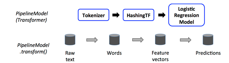
Let’s imagine you are dealing with some classification problems over text documents.

Chances are that your workflow will include the following stages:

1. Split each document into words
2. Convert each word int a vector – you may want to apply some representation model such as Word2Vec
3. Train and compute the prediction of your model

Step 1 requires a Transformer, while Step 2 and Step 3 require to use some Estimators. Through a Pipeline you will be able to aggregate all these steps and to represent them as a pipeline.

A Pipeline is specified as a sequence of stages, and each stage is either a Transformer or an Estimator. These stages are run in order, and the input DataFrame is transformed as it passes through each stage.

For Transformer stages, the transform() method is called on the DataFrame. For Estimator stages, the fit() method is called to produce a Transformer (which becomes part of the PipelineModel, or fitted Pipeline), and that Transformer’s transform() method is called on the DataFrame.

We illustrate this for the simple text document workflow. The figure below is for the training time usage of a Pipeline.

The following image represents the pipeline described above.

A Pipeline works as an Estimator, it means that it has the method fit(). When you call this method on the pipeline, all the stages are executed. More specifically, for any stage S_i we have:

• if S_i is a transformer, the pipeline will call the method transform.
• if S_i is an estimator, the pipeline will first call the fit method and then the transform method

The method fit called on a Pipeline yields a Pipeline model, which is also a Transformer. This means that you can use the this model to call the transform method. As a result, the pipeline will go through all the stages by calling the transform method over each on of them. Be careful that, as opposed to when you called the fit method over the entire pipeline, when you call transform on the Pipeline, all the estimators work as Transformers.

Parameters

You can specify the parameters for either a Transformer of an Estimators in one of the following two ways:

1. Both Estimators and Transformers share a common API to specify their parameters. A parameter is specified via a Param object, which is a named parameter with a self-contained documentation. A ParamMap is instead a set of parameter-value pairs. You can define a ParamMap and pass it to the fit() or the transform() method. A ParamMap is created with the following notation:

   ParamMap(l1.maxIter -> 10, l2.maxIter -> 20)
   

   Where l1 and l2 are two instance included in the Pipeline.

2. Set the parameter directly on the instance that you include within the your Pipeline. Let algo be an instance of any ML algorithm available in MLlib. You can use this instance to set directly the parameters for that particular algoirthm Usually, you have method like set{NameOfTheParameter}.

Examples

• Estimator, Transformer and Param

  import org.apache.spark.ml.classification.LogisticRegression
  import org.apache.spark.ml.linalg.{Vector, Vectors}
  import org.apache.spark.ml.param.ParamMap
  import org.apache.spark.sql.Row
      
  // Prepare training data from a list of (label, features) tuples.
  val training = spark.createDataFrame(Seq(
    (1.0, Vectors.dense(0.0, 1.1, 0.1)),
    (0.0, Vectors.dense(2.0, 1.0, -1.0)),
    (0.0, Vectors.dense(2.0, 1.3, 1.0)),
    (1.0, Vectors.dense(0.0, 1.2, -0.5))
  )).toDF("label", "features")
      
  // Create a LogisticRegression instance. This instance is an Estimator.
  val lr = new LogisticRegression()
  // Print out the parameters, documentation, and any default values.
  println(s"LogisticRegression parameters:\n ${lr.explainParams()}\n")
      
  // We may set parameters using setter methods.
  lr.setMaxIter(10)
    .setRegParam(0.01)
      
  // Learn a LogisticRegression model. This uses the parameters stored in lr.
  val model1 = lr.fit(training)
  // Since model1 is a Model (i.e., a Transformer produced by an Estimator),
  // we can view the parameters it used during fit().
  // This prints the parameter (name: value) pairs, where names are unique IDs for this
  // LogisticRegression instance.
  println(s"Model 1 was fit using parameters: ${model1.parent.extractParamMap}")
      
  // We may alternatively specify parameters using a ParamMap,
  // which supports several methods for specifying parameters.
  val paramMap = ParamMap(lr.maxIter -> 20)
    .put(lr.maxIter, 30)  // Specify 1 Param. This overwrites the original maxIter.
    .put(lr.regParam -> 0.1, lr.threshold -> 0.55)  // Specify multiple Params.
      
  // One can also combine ParamMaps.
  val paramMap2 = ParamMap(lr.probabilityCol -> "myProbability")  // Change output column name.
  val paramMapCombined = paramMap ++ paramMap2
      
  // Now learn a new model using the paramMapCombined parameters.
  // paramMapCombined overrides all parameters set earlier via lr.set* methods.
  val model2 = lr.fit(training, paramMapCombined)
  println(s"Model 2 was fit using parameters: ${model2.parent.extractParamMap}")
      
  // Prepare test data.
  val test = spark.createDataFrame(Seq(
    (1.0, Vectors.dense(-1.0, 1.5, 1.3)),
    (0.0, Vectors.dense(3.0, 2.0, -0.1)),
    (1.0, Vectors.dense(0.0, 2.2, -1.5))
  )).toDF("label", "features")
      
  // Make predictions on test data using the Transformer.transform() method.
  // LogisticRegression.transform will only use the 'features' column.
  // Note that model2.transform() outputs a 'myProbability' column instead of the usual
  // 'probability' column since we renamed the lr.probabilityCol parameter previously.
  model2.transform(test)
    .select("features", "label", "myProbability", "prediction")
    .collect()
    .foreach { case Row(features: Vector, label: Double, prob: Vector, prediction: Double) =>
      println(s"($features, $label) -> prob=$prob, prediction=$prediction")
    }
  

• Pipeline

  import org.apache.spark.ml.{Pipeline, PipelineModel}
  import org.apache.spark.ml.classification.LogisticRegression
  import org.apache.spark.ml.feature.{HashingTF, Tokenizer}
  import org.apache.spark.ml.linalg.Vector
  import org.apache.spark.sql.Row
      
  // Prepare training documents from a list of (id, text, label) tuples.
  val training = spark.createDataFrame(Seq(
    (0L, "a b c d e spark", 1.0),
    (1L, "b d", 0.0),
    (2L, "spark f g h", 1.0),
    (3L, "hadoop mapreduce", 0.0)
  )).toDF("id", "text", "label")
      
  // Configure an ML pipeline, which consists of three stages: tokenizer, hashingTF, and lr.
  val tokenizer = new Tokenizer()
    .setInputCol("text")
    .setOutputCol("words")
  val hashingTF = new HashingTF()
    .setNumFeatures(1000)
    .setInputCol(tokenizer.getOutputCol)
    .setOutputCol("features")
  val lr = new LogisticRegression()
    .setMaxIter(10)
    .setRegParam(0.001)
  val pipeline = new Pipeline()
    .setStages(Array(tokenizer, hashingTF, lr))
      
  // Fit the pipeline to training documents.
  val model = pipeline.fit(training)
      
  // Now we can optionally save the fitted pipeline to disk
  model.write.overwrite().save("/tmp/spark-logistic-regression-model")
      
  // We can also save this unfit pipeline to disk
  pipeline.write.overwrite().save("/tmp/unfit-lr-model")
      
  // And load it back in during production
  val sameModel = PipelineModel.load("/tmp/spark-logistic-regression-model")
      
  // Prepare test documents, which are unlabeled (id, text) tuples.
  val test = spark.createDataFrame(Seq(
    (4L, "spark i j k"),
    (5L, "l m n"),
    (6L, "spark hadoop spark"),
    (7L, "apache hadoop")
  )).toDF("id", "text")
      
  // Make predictions on test documents.
  model.transform(test)
    .select("id", "text", "probability", "prediction")
    .collect()
    .foreach { case Row(id: Long, text: String, prob: Vector, prediction: Double) =>
      println(s"($id, $text) --> prob=$prob, prediction=$prediction")
    }
  

Extracting, transforming and Selecting

This section is organized into three different subsections:

1. Feature Extractors. This section introduces some algorithm for extracting features from your dataset
2. Feature Transformers. This section introduces some of the algorithm that execute commonly used transformations the input dataset

Feature Extractors

• Word2Vec

  Word2Vec is an Estimator which takes as input a sequence of words representing a document and then it trains a Word2VecModel over these words. The model maps each word to a unique fixed-size vector. A document is then represented by simply taking the average of all the vectors associated with any word contained within the original text. Once you have a vector, you can apply all sorts of ML algorithms.

  The following snippet shows how to use this model.

  import org.apache.spark.ml.feature.Word2Vec
  import org.apache.spark.ml.linalg.Vector
  import org.apache.spark.sql.Row
      
  // Input data: Each row is a bag of words from a sentence or document.
  val documentDF = spark.createDataFrame(Seq(
    "Hi I heard about Spark".split(" "),
    "I wish Java could use case classes".split(" "),
    "Logistic regression models are neat".split(" ")
  ).map(Tuple1.apply)).toDF("text")
      
  // Learn a mapping from words to Vectors.
  val word2Vec = new Word2Vec()
    .setInputCol("text")
    .setOutputCol("result")
    .setVectorSize(3)
    .setMinCount(0)
  val model = word2Vec.fit(documentDF)
      
  val result = model.transform(documentDF)
  result.collect().foreach { case Row(text: Seq[_], features: Vector) =>
    println(s"Text: [${text.mkString(", ")}] => \nVector: $features\n") }
  

Feature Transformers

• Binarizer

  Binarization is the process of thresholding numerical features to binary (0/1) features.

  Binarizer takes the common parameters inputCol and outputCol, as well as the threshold for binarization. Feature values greater than the threshold are binarized to 1.0; values equal to or less than the threshold are binarized to 0.0. Both Vector and Double types are supported for inputCol.

  import org.apache.spark.ml.feature.Binarizer
      
  val data = Array((0, 0.1), (1, 0.8), (2, 0.2))
  val dataFrame = spark.createDataFrame(data).toDF("id", "feature")
      
  val binarizer: Binarizer = new Binarizer()
    .setInputCol("feature")
    .setOutputCol("binarized_feature")
    .setThreshold(0.5)
      
  val binarizedDataFrame = binarizer.transform(dataFrame)
      
  println(s"Binarizer output with Threshold = ${binarizer.getThreshold}")
  binarizedDataFrame.show()
  

• PCA

  PCA is a statistical procedure that uses an orthogonal transformation to convert a set of observations of possibly correlated variables into a set of values of linearly uncorrelated variables called principal components. A PCA class trains a model to project vectors to a low-dimensional space using PCA. The example below shows how to project 5-dimensional feature vectors into 3-dimensional principal components.

  import org.apache.spark.ml.feature.PCA
  import org.apache.spark.ml.linalg.Vectors
      
  val data = Array(
    Vectors.sparse(5, Seq((1, 1.0), (3, 7.0))),
    Vectors.dense(2.0, 0.0, 3.0, 4.0, 5.0),
    Vectors.dense(4.0, 0.0, 0.0, 6.0, 7.0)
  )
  val df = spark.createDataFrame(data.map(Tuple1.apply)).toDF("features")
      
  val pca = new PCA()
    .setInputCol("features")
    .setOutputCol("pcaFeatures")
    .setK(3)
    .fit(df)
      
  val result = pca.transform(df).select("pcaFeatures")
  result.show(false)
  

• OneHotEncoder

  One-hot-encoding maps a categorical feature to a binary vector with at most a single one-value. For instance, imagine you have a categorical feature that allows 5 possible categorical values: A,B,C,D,E. This feature is then represented as a 5-sized vector where each value is mapped to a particular position. Therefore the value A - becomes -> [1,0,0,0,0], the value B - becomes -> [0,1,0,0,0] ans so on.

  The following snippet shows how to use this transformer:

  import org.apache.spark.ml.feature.OneHotEncoder
      
  val df = spark.createDataFrame(Seq(
    (0.0, 1.0),
    (1.0, 0.0),
    (2.0, 1.0),
    (0.0, 2.0),
    (0.0, 1.0),
    (2.0, 0.0)
  )).toDF("categoryIndex1", "categoryIndex2")
      
  val encoder = new OneHotEncoder()
    .setInputCols(Array("categoryIndex1", "categoryIndex2"))
    .setOutputCols(Array("categoryVec1", "categoryVec2"))
  val model = encoder.fit(df)
      
  val encoded = model.transform(df)
  encoded.show()
  

StandardScaler

Many ML algorithm are very sensitive to the scale of the input dataset. These algorithms work best when all the feature have the same scale. For this reason it is often required to normalize your data. This scaler normalize the data so that each numerical feature has unit standard deviation and zero mean.

The StandardScaler is actually an Estimator, thus it has the method fit which returns a StandardScalerModel object, which is a Transformer. Therefore, by calling transform on the StandardScaler model you can scale the input features as desired.

The following snippet shows how to use this scaler.

import org.apache.spark.ml.feature.StandardScaler

val dataFrame = spark.read.format("libsvm").load("data/mllib/sample_libsvm_data.txt")

val scaler = new StandardScaler()
  .setInputCol("features")
  .setOutputCol("scaledFeatures")
  .setWithStd(true)
  .setWithMean(false)

// Compute summary statistics by fitting the StandardScaler.
val scalerModel = scaler.fit(dataFrame)

// Normalize each feature to have unit standard deviation.
val scaledData = scalerModel.transform(dataFrame)
scaledData.show()

This is not the only option when it comes to scaling your data. There are other techniques that work the same way as this scaler, the only thing that change of course is the algorithm used for scale the data.

Bucketizer

A Bucketizer transforms a real-valued feature into a column where values are divided into buckets.

When you use this type of transformer you need to specify the buckets into which you wish to divided your feature. Therefore you must specify an ordered vector containing the ranges according to which buckets have to been defined.

The following snippet shows how to use this transformer.

import org.apache.spark.ml.feature.Bucketizer

val splits = Array(Double.NegativeInfinity, -0.5, 0.0, 0.5, Double.PositiveInfinity)

val data = Array(-999.9, -0.5, -0.3, 0.0, 0.2, 999.9)
val dataFrame = spark.createDataFrame(data.map(Tuple1.apply)).toDF("features")

val bucketizer = new Bucketizer()
  .setInputCol("features")
  .setOutputCol("bucketedFeatures")
  .setSplits(splits)

// Transform original data into its bucket index.
val bucketedData = bucketizer.transform(dataFrame)

println(s"Bucketizer output with ${bucketizer.getSplits.length-1} buckets")
bucketedData.show()

val splitsArray = Array(
  Array(Double.NegativeInfinity, -0.5, 0.0, 0.5, Double.PositiveInfinity),
  Array(Double.NegativeInfinity, -0.3, 0.0, 0.3, Double.PositiveInfinity))

val data2 = Array(
  (-999.9, -999.9),
  (-0.5, -0.2),
  (-0.3, -0.1),
  (0.0, 0.0),
  (0.2, 0.4),
  (999.9, 999.9))
val dataFrame2 = spark.createDataFrame(data2).toDF("features1", "features2")

val bucketizer2 = new Bucketizer()
  .setInputCols(Array("features1", "features2"))
  .setOutputCols(Array("bucketedFeatures1", "bucketedFeatures2"))
  .setSplitsArray(splitsArray)

// Transform original data into its bucket index.
val bucketedData2 = bucketizer2.transform(dataFrame2)

println(s"Bucketizer output with [" +
  s"${bucketizer2.getSplitsArray(0).length-1}, " +
  s"${bucketizer2.getSplitsArray(1).length-1}] buckets for each input column")
bucketedData2.show()

VectorAssembler

A VectorAssembler is a transformer that allows you to combine several columns into a single vector column.

It is able to deal with the following column types: numeric, boolean and vector. In each row, the vector is obtained by concatenating the value of each column in the order specified by the user.

The following snippet shows how to use this transformer

import org.apache.spark.ml.feature.VectorAssembler
import org.apache.spark.ml.linalg.Vectors

val dataset = spark.createDataFrame(
    Seq((0, 18, 1.0, Vectors.dense(0.0, 10.0, 0.5), 1.0))
).toDF("id", "hour", "mobile", "userFeatures", "clicked")

val assembler = new VectorAssembler()
    .setInputCols(Array("hour", "mobile", "userFeatures"))
    .setOutputCol("features")
  val output = assembler.transform(dataset)
  println("Assembled columns 'hour', 'mobile', 'userFeatures' to vector column 'features'")
  output.select("features", "clicked").show(false)

Starting from the following situation:

| id | hour | mobile | userFeatures     | clicked |
|:--:|:----:|:------:|:----------------:|:-------:|
| 0  | 18   | 1.0    | [0.0, 10.0, 0.5] | 1.0     |

The above snippet will tranform the dataset as follows:

id	hour	mobile	userFeatures	clicked	features
0	18	1.0	[0.0, 10.0, 0.5]	1.05	[18.0, 1.0, 0.0, 10.0,0.5]

Imputer

The Imputer is an estimator that is useful for replacing missing/null/NaN values accordingly to a predefined strategy. For instance, you might use an Imputer to replace the missing values in a feature of the dataset by replacing them with the average value computed with respect to that feature. An Imputer can only work with numerical features – it is not able to understand categorical values. It also provides the ability to configure which value has to be considered as “missing”. For instance, if we set .setMissingValue(0) then all the occurrences of 0 will be replaced by the Imputer.

The following snippet shows how to use the Imputer.

import org.apache.spark.ml.feature.Imputer

val df = spark.createDataFrame(Seq(
  (1.0, Double.NaN),
  (2.0, Double.NaN),
  (Double.NaN, 3.0),
  (4.0, 4.0),
  (5.0, 5.0)
)).toDF("a", "b")

val imputer = new Imputer()
  .setInputCols(Array("a", "b"))
  .setOutputCols(Array("out_a", "out_b"))

val model = imputer.fit(df)
model.transform(df).show()

Classification & Regression

These are two different types of supervised learning problem.

In any supervised learning problem you are provided with a set of items, each item has a set of features, and more importantly it is assigned with a label.

The type of the label tells you if you are dealing with a regression problem rather than a classification one. More specifically, if the label is a real value then you have a regression problem, while if it is a categorical value then you are dealing with a classification problem.

MLlib offers a lot of algorithms for addressing these kinds of supervised problems. This is the list of algorithms provided by the library:

• Classification
  • Logistic regression
    • Binomial logistic regression
    • Multinomial logistic regression
  • Decision tree classifier
  • Random forest classifier
  • Gradient-boosted tree classifier
  • Multilayer perceptron classifier
  • Linear Support Vector Machine
  • One-vs-Rest classifier (a.k.a. One-vs-All)
  • Naive Bayes
  • Factorization machines classifier
• Regression
  • Linear regression
  • Generalized linear regression
    • Available families
  • Decision tree regression
  • Random forest regression
  • Gradient-boosted tree regression
  • Survival regression
  • Isotonic regression
  • Factorization machines regressor
• Linear methods
• Factorization Machines
• Decision trees
  • Inputs and Outputs
    • Input Columns
    • Output Columns
• Tree Ensembles
  • Random Forests
    • Inputs and Outputs
      • Input Columns
      • Output Columns (Predictions)
  • Gradient-Boosted Trees (GBTs)
    • Inputs and Outputs
      • Input Columns
      • Output Columns (Predictions)

We will not discuss any of the previous algorithms. Since this is beyond the scope of this lesson. A useful resource to learn (quickly) is the scikit-learn documentation, available here.

Model Selection and Tuning

This section describes how to use MLlib’s tooling for tuning ML algorithms and Pipelines. Built-in Cross-Validation and other tooling allow users to optimize hyperparameters in algorithms and Pipelines.

Parameter Tuning

Parameter Tuning is the task of trying different configuration in order to improve performance.

You can tune a single estimator as well as an entire pipeline. When you want to improve the performance of your model you need an object of type Evaluator. An Evaluator allows you to evaluate how well your model is able to fit the data. There is a number of different evaluators, the right one depends on the type of problem you are dealing with. For instance if you are dealing with a regression problem you should use the RegressionEvaluator, while for classification problems you should use the BinaryClassificationEvaluator or the MulticlassificationEvaluator.

A common way tune an ML model is by defining a grid, which determines the range of values a particular parameter can assume. This kind of behavior is achieved via the ParamGridBuilder object. A grid based tuning works as follows. Imagine your model M has depends on two different hyperparameters: p₁ and p₂. You define a range of values for each one of them. For instance you may specify that p₁ varies within the range [0,10] with step 2, while p₂ varies within the range [-10, 10] with step. This means that you would have 5 different possible configuration for p₁ and 3 different configuration for p₂. In this case your model will be trained 5x3=15 different times, assessing every possible configuration with respect to both parameters.

Cross Validation

Another important technique for selecting the best model is the Cross-Validation. In order to train your model with the cross-validation there is an object called CrossValidator. A CrossValidator is actually an Estimator, so you can call fit and then you get a model. The following snippet shows how to use the a CrossValidator.

...
val tokenizer = new Tokenizer()
  .setInputCol("text")
  .setOutputCol("words")
val hashingTF = new HashingTF()
  .setInputCol(tokenizer.getOutputCol)
  .setOutputCol("features")
val lr = new LogisticRegression()
  .setMaxIter(10)
val pipeline = new Pipeline()
  .setStages(Array(tokenizer, hashingTF, lr))

// We use a ParamGridBuilder to construct a grid of parameters to search over.
// With 3 values for hashingTF.numFeatures and 2 values for lr.regParam,
// this grid will have 3 x 2 = 6 parameter settings for CrossValidator to choose from.
val paramGrid = new ParamGridBuilder()
  .addGrid(hashingTF.numFeatures, Array(10, 100, 1000))
  .addGrid(lr.regParam, Array(0.1, 0.01))
  .build()

val cv = new CrossValidator()
  .setEstimator(pipeline)
  .setEvaluator(new BinaryClassificationEvaluator)
  .setEstimatorParamMaps(paramGrid)
  .setNumFolds(2)  // Use 3+ in practice
  .setParallelism(2)  // Evaluate up to 2 parameter settings in parallel

val model = cv.fit(data)

Anatomy of a ML application

Any ML application should adopt the following development steps:

• Think about the problem you are interested in. You should ask yourself the following questions:
  • How would I frame it?
  • Is it a supervised problem? Is it better to address the problem as a classification problem rather then a regression one?
• Get the data. In this stage you get the data required to solve the problem you are interested in.
• Analyze your data, compute summary statistics, plot the data, gain insights.
• Prepare your data to apply ML algorithms. In this stage you apply transformer to clean your data – for instance you can apply the Imputer to replace missing value –, or you can apply transformer to obtain a different representation of your data – for instance Word2Vec or OneHotEncoding.
• Split your dataset. You must always remember to reserve a fraction of your data to validate your model. It means that you must split the data (at least) into training and test set. The training set is used to train your model, while the test is used to understand how godd is your model in terms of generalization
• Select the most promising models and apply parameter tuning on them
• Present the results