Diagnostic & Debugging

If you have hard time in minimizing the cost function of your learning algorithm, you should give it a try to one of the following solutions:

• increase the number of data points
• try to focus on a subset of the original features
• try to add more features (e.g., some linear combination of the existing features)
• play with different regularization terms

Which is the right option?

It depends! In order to understand the most profitable option among above directions requires you to perform a diagnosis of your ML algorithm.

Diagnostic can guide you to select the most effective strategy to improve the performance of your algorithm.

Performance Evaluation

There are two main scenario to avoid:

• Overfitting
• Underfitting

A standard approach is to split your dataset into two disjoint sets.

The largest fraction of your data has to be reserved to the training set. The amount of data in your training set is roughly about the 30% of the entire daatset. It is also recommended to shuffle your data before executing the splitting.

Once you have split the data you can compute two cost functions, denoted by:

• J(Θ) - Value of the cost function on the training set
• J_test(Θ) - Value of the cost function on the test set.

Θ denotes the parameter vector that characterize your hypothesis – hereinafter denoted by h_Θ, i.e., your model.

Usually, J(Θ) and J_test(Θ) are the same function. However, they can also be different from each other.

For instance, in the context of (binary) classification, your model minimize the following function:

But you can use the mis-classification error to evaluate the performance on the test set. More formally, given a data point x, the error is defined as:

Where ŷ denotes the value predicted by your model.

Finally, the total error is obtained by summing the above function upon each data point in the test.

The Model Selection Problem

Usually – not necessarily – the error computed on the test set will be higher than the one obtained on the training set.

The error on the test set is referred as generalization error.

Your goal as a data scientist is to provide a model with the lowest generalization error.

However, you are not supposed to select your best model based on the performance achieved on the test set.

Imagine you have to train a model upon different representations of your original dataset.

For instance, you can have several polynomial representations by changing the order of the polynomial.

Degree	Hypothesis
1	hΘ(x) = θ0 + θ1x1
2	hΘ(x) = θ0 + θ1x + θ2x2
3	hΘ(x) = θ0 + θ1x + θ2x2 + θ3x3
.	.
.	.
10	hΘ(x) = θ0 + θ1x1 + θ2x2 + … + θ10x10

Clearly, each polynomial representation leads to a different hypothesis (i.e., Θ⁽¹⁾, Θ⁽²⁾, …, Θ⁽¹⁰⁾).

At this point we need to establish which is the best model among the above 10 different hypothesis.

A pitfall to avoid is to establish the best model based on the test error. In fact, the test error is often an optimistic estimate of the true performance of our model.

Therefore, in the above scenario, we cannot decide which is the best choice for the degree of the polynomial representation based on the performance on the test of each model.

This is wrong because it is like we were trying to fit the test set!. The test set is only meant to report the generalization error, you are not supposed to take any design decision based on the above error.

The validation set

In order to solve the above problem, you can split the data into three separate sets.

Typically, the training set takes roughly the 60% of the entire dataset, the remaining part is equally divided between the validation and the test set.

Now for each of the above hypothesis you should also evaluate the cost function with respect to the new validation set (J__val(Θ))

For instance, if you have the following situation (J(Θ) is an arbitrary cost function).

Degree	Hypothesis	J(Θ)	(J_val(Θ)	(J_test(Θ)
1	hΘ(x) = θ0 + θ1x1	.5	.6	.65
2	hΘ(x) = θ0 + θ1x + θ2x2	.23	.5	.43
3	hΘ(x) = θ0 + θ1x + … + θ3x3	.2	.3	.45
4	hΘ(x) = θ0 + … + θ4x4	.2	.2	.39

Based on the above results you should decide that the 4th model is the best option. The test set error is reported only as an estimate of the generalization error.

With this approach we ensure that J_test(Θ) is a more accurate estimate of the actual generalization error, since it did not play any role in the decision related to the best model.

Take Home Lesson

• The test set error should not play any role in the model selection
• The only purpose of the test set error is to provide an (optimistic) estimate of the generalization error
• Always split your data into Training/Validation/Test Set error.

Bias vs Variance

Bias and variance are the reasons underlying your model underfitting or overfitting the data.

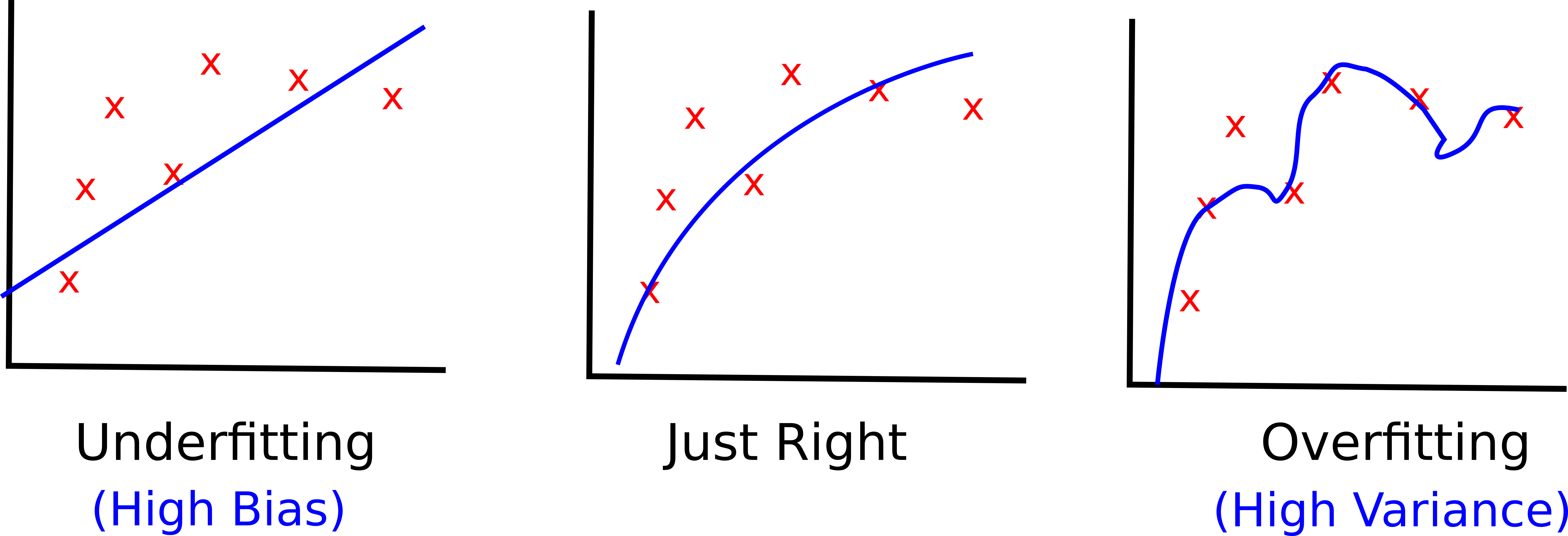
Typically, when your model underfits the data means that it has too high bias. Conversely, when your overfits your data means that it has too high variance.

More formally, we can define bias and variance as follows.

• Bias Error - it is the error derived from erroneous assumptions made by your learning algorithm (e.g., a linear regression implicitly assumes that a lines can fit your data).
• Variance Error - it is the error derived from the fluctuations in your training set (e.g., a powerful neural network might be able to fit the noise in your training data).

At a high level, the goal of any learning algorithm is to minimize both the bias and the variance error.

Unfortunately, improving on one error is likely to have a negative impact on the other error. This is often referred as the bias-variance dilemma!.

Let’s consider the above example on the polynomial representation of your data.

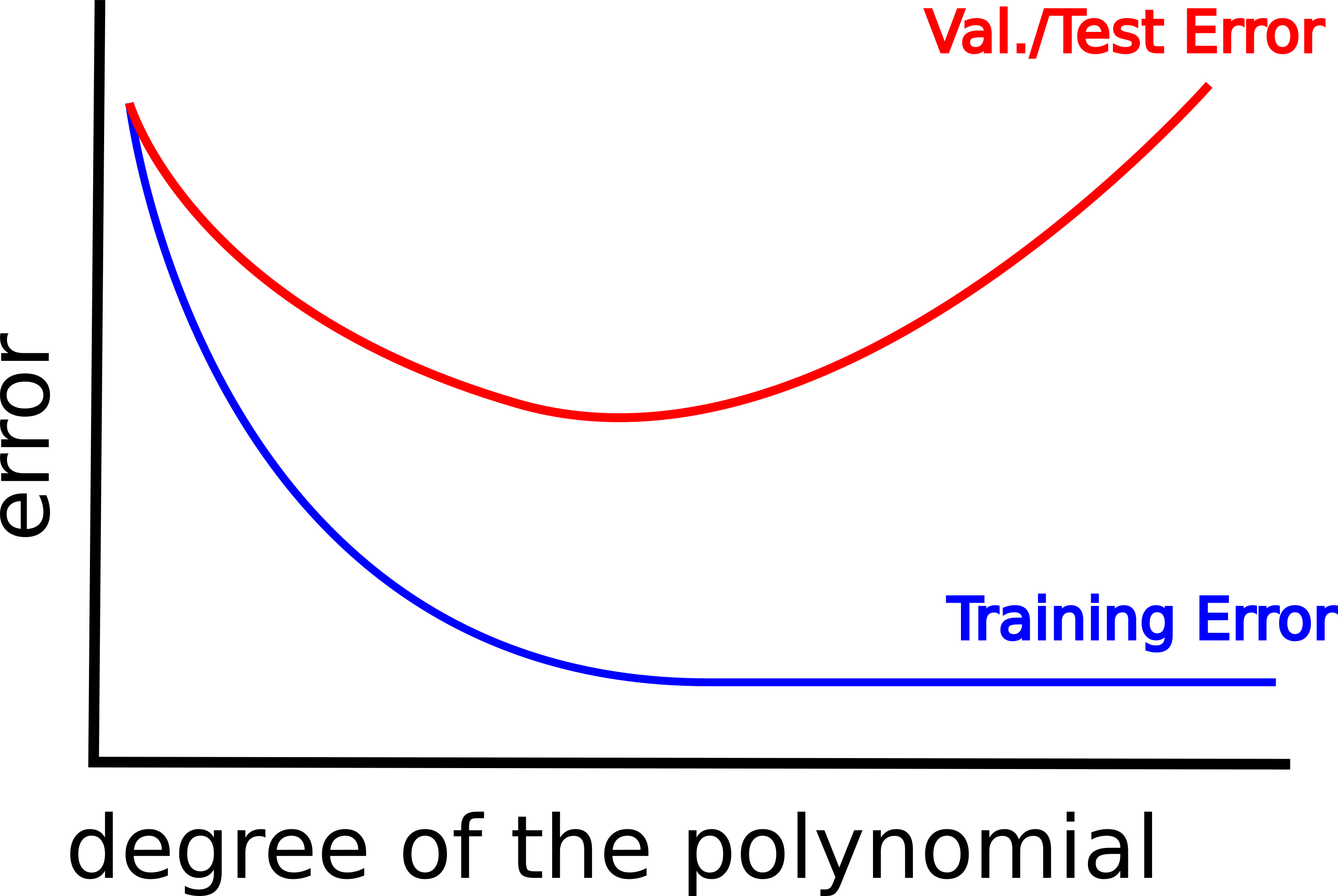
The above image suggests that as the degree of the polynomial increases, the training error progressively decreases.

Conversely, the validation error tends to decrease at first, but when the degree of the polynomial goes beyond a certain threshold it tends to significantly increase.

When you have a high test/validation error it means that your are in either one of the two situations highlighted by the purple circle in the figure below.

Specifically, if your are in the situation corresponding to the left side of the figure, then your high test/validation error can be ascribed to your model suffering from a high bias problem (i.e., the model is not powerful enough to fit the training data).

On the other hand, the right side of the image corresponds to a high variance problem (i.e., your model is so powerful that it is able to fit the noise in the training set).

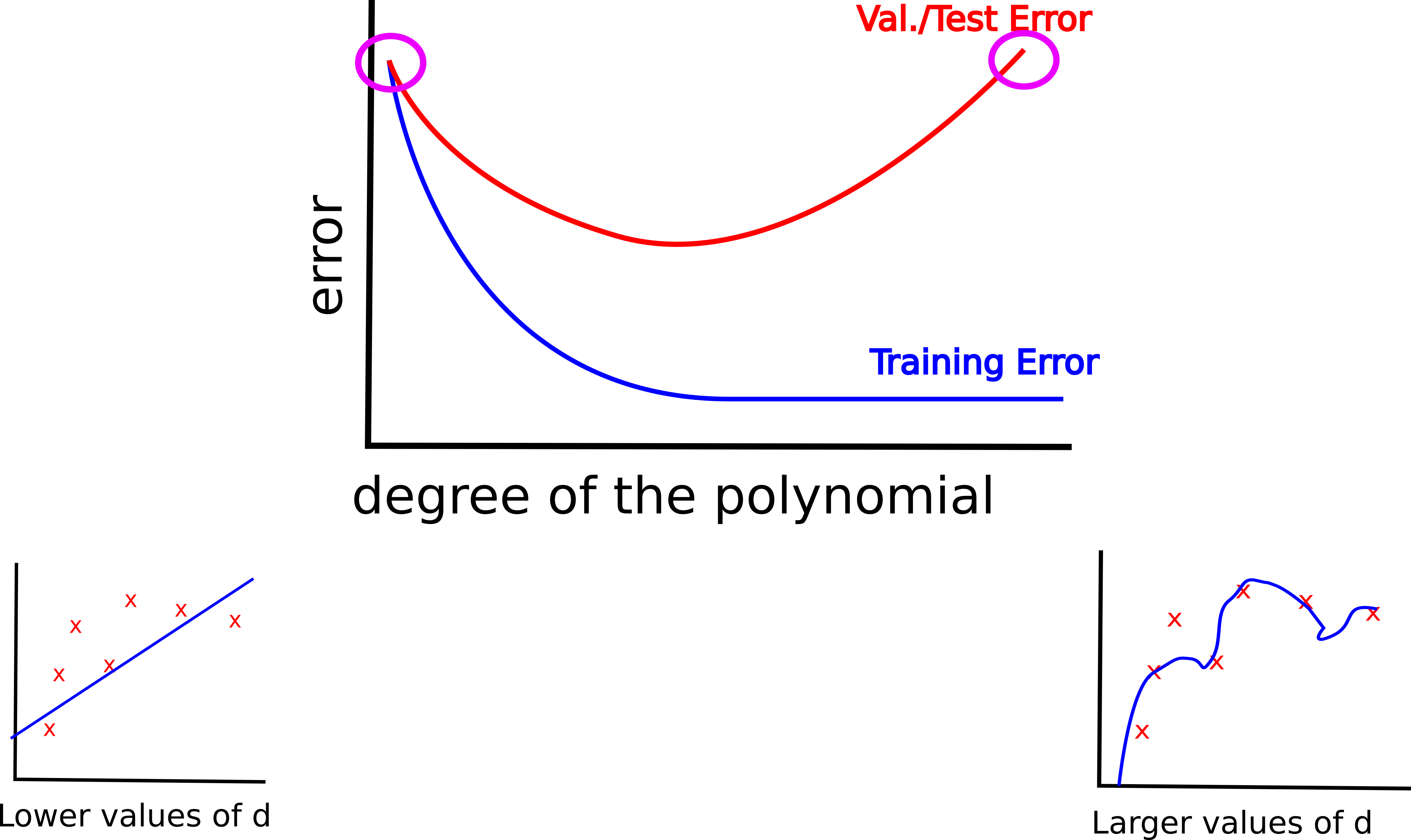
How to distinguish between the two situations?

• In the first scenario – leftmost circle – the training and test error are both very high. In this case, you should try with a more powerful model.
• In the second scenario – rightmost circle – the training error is kept low, but there is a significant difference with the test/validation error. In this case you should try to regularize your algorithm.

The impact of regularization

Imagine you decide to use a powerful model to fit your data, let’s say you are using a pretty powerful, cocky, deep neural network.

Clearly, neural networks might suffer from a high variance problem, since they are very powerful. Therefore, you need a strategy to prevent them to overfit the training data.

This is indeed the goal of regularization. Concretely, when you use regularization, the cost function used during the training phase accounts for an additional parameter, i.e., the regularization term.

Therefore, the cost function is defined as follows:

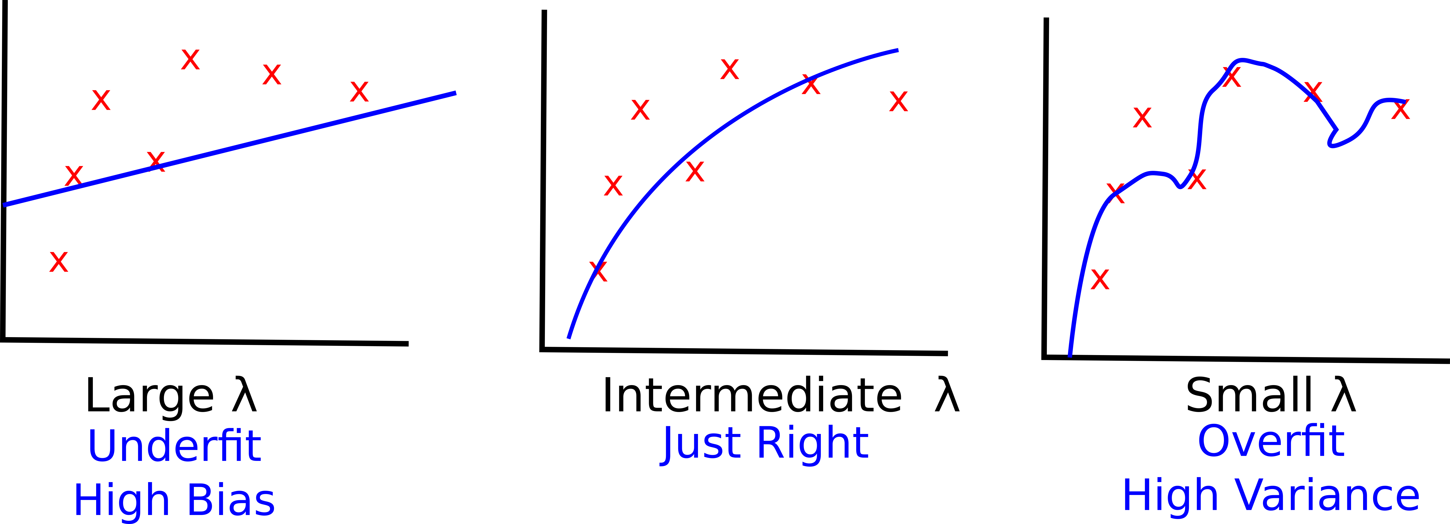
The effect of the regularization term is to constrain the variance of the learning algorithm. The value of λ determines how much you want to penalize the weights of your hypothesis.

Let’s see the impact of the regularization term on the learned hypothesis.

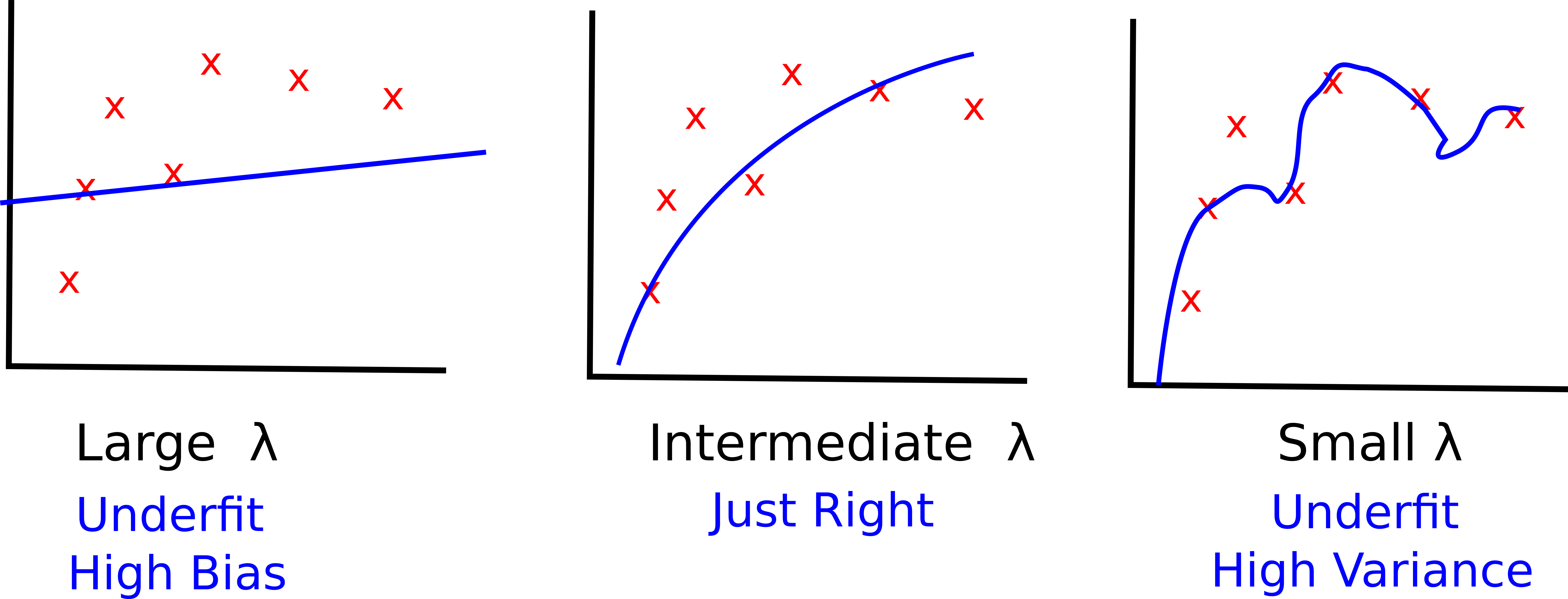
• Larger values of λ increase the chance of underfitting the data, thus they introduce a higher bias. In the rightmost figure, most of the parameters of your hypothesis are close to 0
• Smaller values of λ increase the chance of overfitting the data, they introduce a higher variance in your learning model. In the leftmost figure the effect of the regularization term is almost negligible

How to choose the right value for λ? Similarly to the model selection problem you should let the validation error guide your selection.

A meaningful range of value to try is the following.

Model	λ
Θ(1)	0
Θ(2)	0.01
Θ(3)	0.02
Θ(4)	0.04
.	.
.	.
Θ(12)	10

Each model is trained by minimizing the cost function plus the regularization term.

Finally, you can compute the validation error with respect to each possible configuration of λ and then you select the regularization term that provided the best performance on the validation set.

A pitfall to avoid is to use the regularized cost function to report the error on the validation set. In fact, the regularization term introduce a competitive advantage in favor of the models trained with higher values of λ

Therefore is you use the following function during training.

Then you should use the following cost function for the validation and the test set.

Let’s focus on the impact of the regularization term on the bias/variance trade-off.

Clearly, the best choice for lambda is the one highlighted by the dashed line in the above image. In fact, the corresponding value of λ provides the lowest validation error.

Learning Curves

Plotting the learning curves of your algorithm is another useful tool to spot the presence of underfitting or overfitting.

With learning curves you are able to understand which is the benefit of bringing new data to your problem. In fact, here we focus on the value of the training and val/test error as a function of the number of data points available to your learning algorithm.

In order to derive the learning curves of your algorithm you can train the algorithm on a progressively larger portion of your training data.

This is a possible approach:

1. Select m data points
2. Train your data on the first m data points of your training set
3. Plot the J(Θ) and J_val/test(Θ) with respect to the entire first m training points and test/validation set, respectively
4. Increase m and go to 1

Clearly, when you have few data points your model will be able to fit them all without any particular problem. However, as the number of points increases, it will be harder for your model to fit all the data, as a consequence the training error will increase.

This is how the learning curves look like on a “wealthy” model.

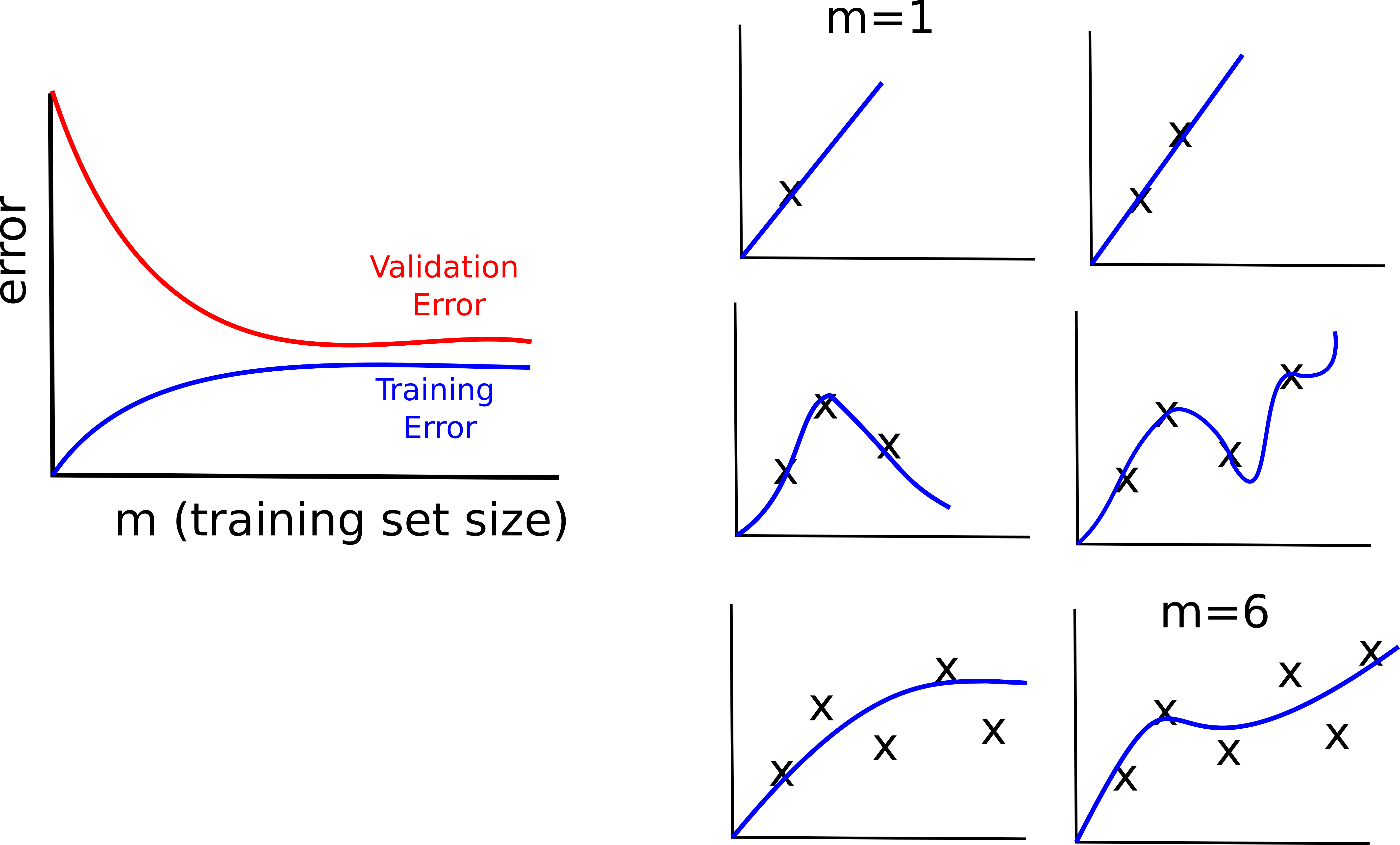
We can say that this model well behaves for the following reasons:

• the training error and the validation error are very close to each others. It means that the model does not suffer from overfitting
• both the training error and the validation error are relatively low. It means the model does not suffer from underfitting

High Bias

If your model suffer from high bias, it means that it tends to underfit the data. In this case, the learning curves will look as follows.

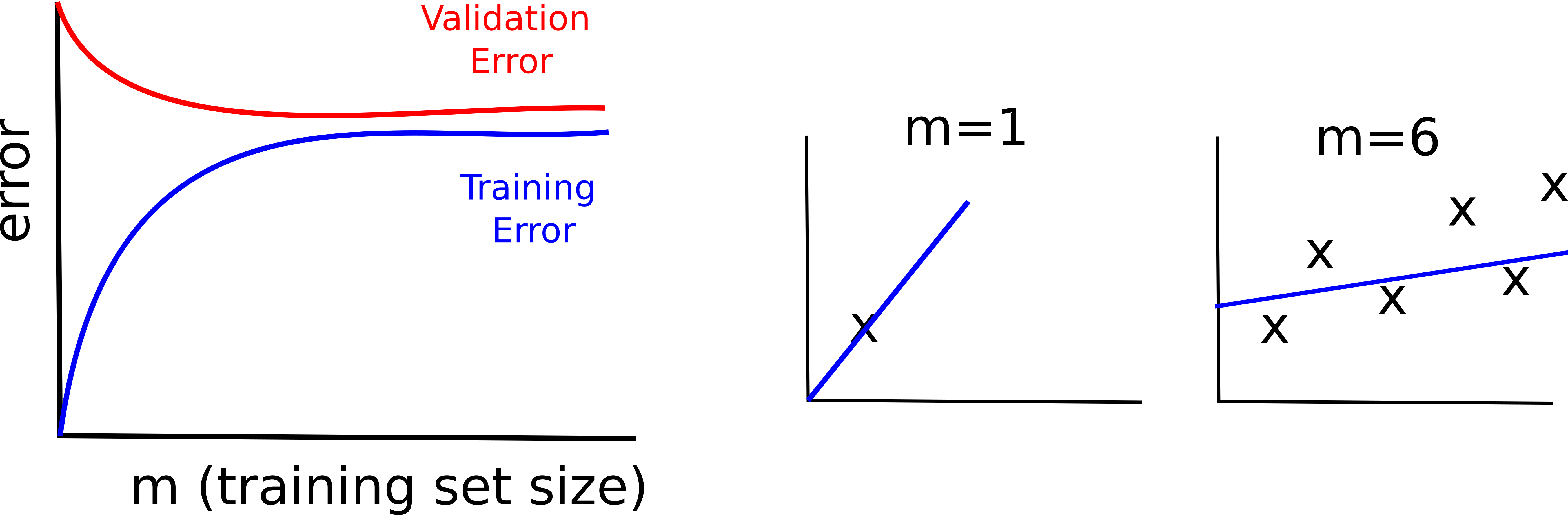
• both training and validation error are pretty high
• the benefit of adding new data points becomes negligible very soon (your model is not able to learn from the data)

High Variance

If your model suffer from high variance, it means that it tends to overfit the data. In this case, the learning curves will look as follows.

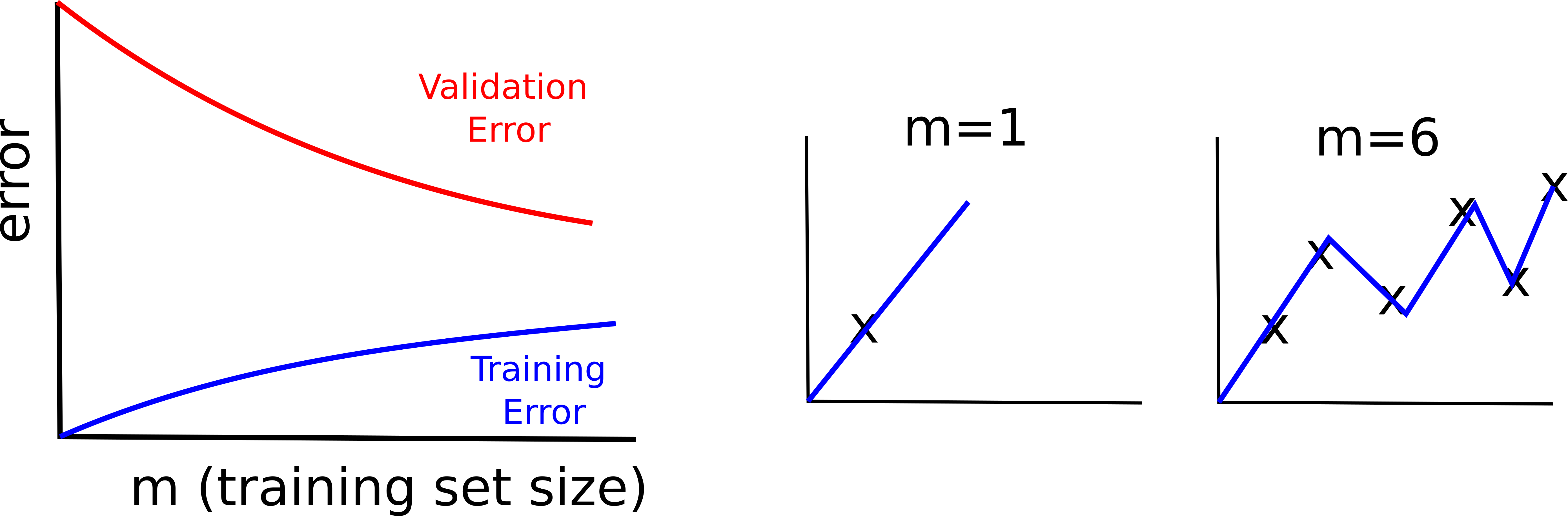
• the difference between the training and the validation error is significant
• the training error grows slowly with the amount of training data, while the validation error continues to decrease

Recap

Going back to the question at the beginning of this lesson: which is the best strategy to improve the performance of your algorithm when you are having hard times in minimizing the cost function?

High Bias	High Variance
Try to get additional features	Get More Training Examples
Try decreasing the reg. term	Try with a reduce set of features
	Try increasing the reg. term

Use Case: Spam Classifier

You are required to build a Spam classifier, namely a model that takes as input the vector representation of an email and it output:

Data Engineering

The first problem to address is to decide how to represent an email. p A possible solution would be to determines a set of words – the most frequent k (top-k) – so that we can map an email to a {0,1} vector of k positions.

How to proceed from here?

• You can collect more data
• Design more sophisticated features
  • We can encode the information related to the email routing, contained in the header of an email
  • Apply text-based preprocessing techniques. For instance, you can use methods to detect semantic analogies; you can use design features based on the punctuation of the text

Error Analysis

Unfortunately, there is no way to tell which of the above strategies will prove to be the most effective. Therefore, the most reasonable thing to do is error analysis.

The recommended approach is the following:

1. Start with a simple algorithm and test its performance on the validation set
2. Plot the learning curves to spot the presence of high-bias or high-variance
3. Perform Error Analysis. Manually examine the examples in the validation set that your algorithm made errors on. See if your are able to spot any systematic trend in the type of examples it is making errors on.

For instance, imagine that your algorithm misclassifies 100 emails over the 500 examples in the validation set.

You should manually examine the 100 errors and the categorize them based on aspects such as:

• the type of email (e.g., reply email, password reset emails, pharmaceutical)

Then you should ask yourself: what features would have helped the algorithm to classify them correctly?

The answer to the above question could lead to the definition of the following features:

Feature	Description
Pharmaceutical	Is the email related to some drug?
Reset Password	Is the email asking you to insert a password?
Number of mispellings	Medicine becomes med1cine, mortgage becomes m0rgage
Unusual punctuation	The email uses a lot of !!!!!! or ??? and other unusual symbols

This analysis is arguably a valuable tool. However, sometimes it is hard to understand how to define new features in order to help your classifier.

For instance, error analysis is not able to suggest your whether or not stemming will increase the performance of your algorithm.

In these situations the best strategy to adopt is based on trial-and-error. In order to understand if a given technique is able to improve the performance of your algorithm you should always assess its effectiveness on the validation set.

Example

• Should you use stemming?
  • Compute the validation error with and w/o stemming
• Should you use distinguish between upper and lower case?
  • Compute the validation error with and w/o distinguish between upper and lower case